Deep Learning Textbook Chapter 1: Linear Algebra
May 12, 2016

The Dolan lab group (and friends) is working through the soon-to-be-released Deep Learning textbook, authored by Goodfellow Bengio, and Courville, and somewhat miraculously available in html form prior to publication by MIT press.
At a risk of exposing the depths of my ignorance to the internet, I’m going to try and publish my notes on each chapter of the book online here, along with related resources which I found useful. Naturally, these will be somewhat idiosyncratic and by no means authoritative; the craters in my understanding may not align with your own. Thanks to Zeb & Anish for checking the below.
Some notation
BOLD CAPITALS are matrices e.g. A
lowercase bold are vectors e.g. a
lowercase are scalars e.g. a
Some terms
Broadcasting: repeated use of a vector, such as when adding a vector to a matrix using the shorthand C = A + b; the vector is repeated to fill the unspecified dimension (i.e. if matrix is m x n and vector is m x 1, b is essentially repeated n times).
Different multiplications
For vectors:
Inner product:
A helpful way of remembering this is that the inner dimensions are the ones that have to match – hence, inner product. So an [1,m] vector x [m,1] vector gives you a single number – we basically do this between every row and every column when we do a matrix product (see below).
A useful geometric addendum; the product between two vectors is equivalent to their norms (see below – basically their lengths), multiplied by the cosine of the angle between them:
Which means that if the two vectors are orthogonal, theta=90, and cos(90) = 0, therefore:
For matrices:
Standard matrix multiplication:
Matrix 1 (m,n) x Matrix 2 (n, p) = Matrix 3 (m, p).
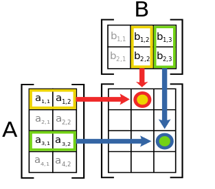
This is a matrix version of the vector inner product (see above). Remember that we have to match the ‘inner dimensions’ – so an m x n matrix can be multiplied by an n x q matrix. These two matching dimensions then ‘fuse’ to give you an output which has the number of rows of the first matrix (m), and the number of columns of the second (q).
Here’s a neat wikipedia graphic as an aid to those of us with dubious mathematical memory (or who are too reliant upon matlab) how to actually obtain your matrix product:
Hadamard product:
Taking the element-wise product of two matrices. Just take the two numbers in equivalent positions in either matrix, multiply them together, and your done. This is probably what you did the first time you tried your hand at matrix multiplication.
Thinking about vectors as points and matrices as transformations
Zeb thinks about vectors as points in space (with dimensions = number of rows), and matrices as transformations. This has turned out to be a useful mental model for me. A video demonstration of how a matrix can be used to transform a vector comes from the indubitable Khan academy.
Why does this make sense? Because we know from our matrix multiplication rules that if we take the product of a matrix and a vector where the matrixhas dimensions [m,m] and the vector has dimensions [m,1], then we get out another vector which has dimensions [m,1] – which is the same dimensions as the vector we started out with! So we’ve transformed the original vector.
Linear combinations and span
An important and, for me, not utterly intuitive point. If we have a matrix with dimensions [m,m], we can use linear combinations of those columns to define any point in a space with m dimensions, assuming the ranks and columns of the matrix aren’t redundant with one another.
What?!
This video does a nice job of explaining it (again, Khan academy leads the way). Here’s how to think about it
- Let’s say we have a matrix with two columns and two rows; so m=2, n=2. Let this matrix be M
- We can define linear combinations of those columns: so a x M(:,1) and b x M(:,2), and we can set a and b to whatever we want. Now the surprising thing is that, if M(:,1) and M(:,2) aren’t redundant with one another – meaning that we can’t transform one into the other by using a scalar, like a or b – then some mixture of M(:,1) and M(:,2) can define ANY POINT in a 2 dimension space.
- This is a little hard to believe without seeing a few examples
- A good analogy: if you can only walk forwards/backwards (column 1) and left/right (column 2), then you can reach any point on a 2D plane. This is exactly the same idea. In a redundant matrix, we have something equivalent to column 1 = forwards/backwards, column 2 = backwards/forwards or something like that.
Note that this doesn’t work if any of the matrices columns or rows can be obtained by a linear combination of the other columns (so the suspect column doesn’t really represent a new direction).
The rank of the matrix is thus the number of unique rows or columns, whichever is smaller (there are some proofs which show that the matrix rank == column rank == row rank).
The span of a matrix is the set of points obtainable by a linear combination of the matrix’s columns. If all of the columns are independent, then the span incorporates all points in a n-dimensional space, where n is the number of columns.
If that doesn’t make sense, seriously, go and watch the Khan academy video, it’s excellent.
Identity and inversion
Identity matrices are simple: matrices which you can multiply a vector by and achieve… nothing. They are all zeroes apart from the diagonal (matlab command eye(n)).
The inverse of a matrix is the matrix whose multiplication with the original produces the identity matrix:
[equation]
This is useful because it allows us to solve equations of the form
[equation]
Where we’re interested in a vector b which offers a solution to the projection of vector x through matrix A. Using the definition of the identity matrix, we can multiply both sides by the inverse, use the definition of the identity matrix above, and get:
[equation]
Linking this up with the discussion of span above: the matrix inverse ([equation]) exists if there is a unique b for every x. For this to be true, every b must be in the span of A. From the discussion above, this induces a very fundamental constraint, namely that b cannot have more dimensions than A has non-redundant columns. A simple way of thinking about this: if b is some point in 3D space, but we can only trace out a 2D space using our matrix columns, then our estimate of b forms a 2D plane in a 3D space; the true value of b could be anywhere on that plane and we would have no idea where it was in the third dimension.
What about the number of rows? It turns out that this matters too. If m>n (we have more rows than we have columns), then we have more dimensions than we have directions, and the solution is once again indeterminate. To be completely honest, I haven’t plugged through any examples to get a deep intuition of why this is. Returning to the forwards/backwards, left/right analogy employed above, I guess that it makes sense that we would need a third possible direction in order to find all the points in a 3D space?
And so we have arrived at a recipe for an invertible matrix:
- It’s square (m=n)
- It has linearly independent columns (this is called [in a confusing negative fashion] being not singular).
Matrices which we can’t invert due to linear dependence between columns are called singular or degenerate matrices.
Phew.
Norms
Norms are ways of measuring the lengths of vectors. Norms are denoted using double lines: ||A||. In the very general sense, a norm is defined as:
What we choose as p determines what kind of norm it is. You hear about norms a lot in the context of regularisation in machine learning, where we have to decide how much to punish the weights on a neural network in order to prevent overfitting.
Common ones:
L2 Norm Where p=2, is the Euclidean norm. It’s basically just the distance of a vector from the origin. L2 norms promote low values of parameters if used for regularisation.
Typically, people square the L2 norm (so we have s ort of L2^2 norm). This lends some mathematical tractability (apparently). Now the problem with this is that the squaring operation means that when we’re close to the origin (x is very small), we get very small changes. This isn’t great for various applied reasons in machine learning. So we turn to the
L1 Norm which is just the absolute value of a vector – the sum of the components. This has the useful property that it changes at the same rate regardless of where we are in the space; so a change from [3 4] to [4 5] is a change of 2, as is a change from [55 56] to [56 57]. The L1 norm promotes sparseness in regularisation – we tend to get lots of zero valued parameters.
Max norm: absolute value of the element with the largest value in a vector
Frobenius norm: this rather esoteric chap is like the L2 norm but for matrices: it’s the (square root of) the sum of the square of all the elements:
Eigendecomposition
A phrase which still chills my blood slightly.
A great deal of insight can be achieved by returning to the notion that a matrix is a transformation. With this held in mind, an eigenvector is merely a vector that can undergo this transformation whilst changing only it’s scale, not its direction.
Where [equation] is the eigenvalue and v is the eigenvector.
A matrix can have multiple eigenvectors, with associated eigenvalues.
Why do we care? A neat analogy adopted by the textbook is that we gain insight from decomposing matrices into eigenvalues and eigenvectors in much the same way that we gain insight into whole numbers by decomposing them into their factors.
This is an amazing interactive webpage exploring eigenvalues and eigenvectors. One point it makes, which I hadn’t grasped, is that eigenvectors represent the attractors of a repeating system: if we repeatedly multiply a matrix by a vector, we will eventually end up on one of the eigenvectors of that matrix!
Another property suggested by the above: if your largest eigenvalue=1**, you converge upon a steady-state system,** whereby repeated multiplication of the eigenvector by the matrix produces no change.
Singular value decomposition (SVD)
In applied maths/science, you hear more about SVD than you do about eigendecomposition. The intuition is the same; it’s a way of breaking up a matrix into its fundamental parts, and thus getting a handle on which components are important. It’s often used, for instance, in image analysis to remove noise components.
The SVD is more general than eigendecomposition. It works for non-square matrices. it consists of breaking up our source matrix into three matrices:
[equation]
If A has dimensions m,n, then U is (m x m) and V (n x n) are defined to be orthogonal. D is a m x n diagonal matrix, and the values along this diagonal are the singular values.
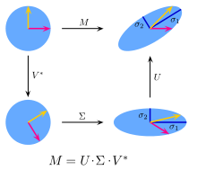
Wikipedia has a different notation, which means the same thing, and is accompanied by a nice graphic:
This articulates the idea that each component matrix can be thought of as applying a different part of the total transformation (M), which is a rotation and a stretch. Breaking this up, V* does a rotation, [equation] does a stretch, and U does another rotation.
Determinants
These seem incredibly hard to quantify, but capture the ‘volume’ of a matrix. It’s also equal to the product of the eigenvalues. One function is to describe how the matrix changes the size of vectors which are multiple by it.
A matrix whose determinant is 1 does not change the size of vectors by which the matrix is multiplied. Conversely, a matrix with a determinant of 0 collapses one dimension to zero. This may remind you of the row-deficiency problem described earlier (‘we don’t have enough dimensions in our matrix, so we end up with an unspecified dimension’)… sure enough, matrices which are rank-deficient have a determinant of 0 (one way of thinking about this: these matrices occupy ‘flat’ spaces – and flat things have a volume of 0!).
Principal Components Analysis (PCA)
PCA is dealt with at the end of this chapter – but a much better treatment of the topic than I could possibly offer can be found here, at the blog of somebody far more mathematically proficient than I.


