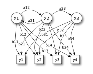
Deep Learning Textbook Chapter 2: Probability

May 19, 2016

As part of the Max Planck Centre’s Deep Learning reading group, I’m working my way through the soon-to-be released Deep Learning textbook. These posts are my informal notes for each chapter. Find my notes from chapter 1 here. Thanks again to Zeb & Toby for edits.

This week we were back on slightly firmer ground, dealing with the chapter on probability. Most of this chapter will be fairly familiar to those who have done some statistics and/or computational modelling. My notes are correspondingly sparse.

Flavours of uncertainty in modelling

Inherent stochasticity, e.g. in the outcome of a coin flip (equivalent to irreducible uncertainty, which we wrote about here)
Incomplete observability – we don’t have enough information to fully specify what’s going to happen
Incomplete modelling – all models are wrong, some are useful (George Box). All models sacrifice some precision in order to make useful simplifications of the subject under study; these simplifications bring with them some uncertainty.

Frequentist vs Bayesian probability

The textbook has a nice delineation of two ways of thinking about probability.

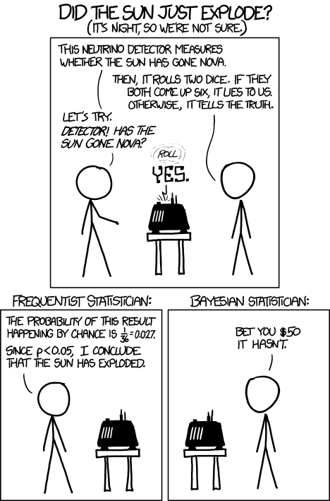
The frequentist tradition maintains that probability is the percentage of times that something has happened divided by all the times it might have happened, and, in the strongest interpretation, that these are the only kind of probabilities it makes sense to talk about. We can therefore derive probabilities for rain on a day in June, but we can’t derive probabilities for the likelihood of the sun exploding, or for the probability of my having cancer.

A Bayesian treatment, however, allows us to use probabilities to describe various degrees of certainty, or degrees of belief. This is far more useful from a neuroscientific perspective, and allows us to do all sorts of neat stuff, like integrate sensory information optimally or learn at appropriate rates.

Bayesian statistics also allows us to integrate priors – information about how likely something is, a priori (that is, without observing any new information). This can be pretty useful:

Probability Mass Functions

A Probability Mass Function (PMF) describes the probability of a randomly drawn sample from x taking on a certain value x (note the italics) : P(x=x).

PMF’s are used when variables are discrete. They generate nice blocky histograms, with the height of the bar telling us how likely we are to observe that value of x. For instance, this is the PMF for a (fair) die:

Probability Density Functions

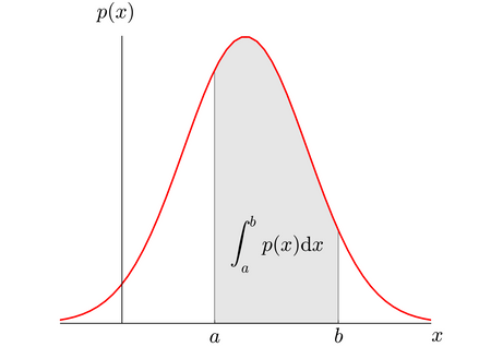
Probability Density Functions (PDF’s) deal with the P(x=x) again, but for continuous variables. This has one huge implication: the height of the function no longer tells us the probability of observing that particular value of x, as the probability of seeing x of a particular value ~=0. This is because the function is continuous – so it has infinitely many values – and since the probability of any one value is going to be 1 / n_possible_values, we have 1/infinity == 0.

Intuitively, this is not different from the material meaning of density – if we take an infinitely small volume, we can’t say anything about its density (since density = mass/volume). We need to specify a volume in order to measure the density and therefore infer the mass.

Instead, we use integration with some set of limits to tell us how likely we are to observe x in some range. So we can ask: ‘how likely am I to observe x between a and b?’:

Marginal probabilities

We use marginal probabilities to isolate the probabilities of a subset of variables. Say we have a bunch of people, and we split them up according to gender and by height. We now have them labelled as short/tall, and male/female, and we count them as

30 tall men

15 short men

20 tall women

35 short women

Now if we want to know the probability that a random draw will produce a man, we can marginalise over the height variable to find p(male):

Where X is male/female, and Y is tall/short. In order to isolate the probability distribution of gender, we need to ‘sum out’ the probability that the person is tall or short.

Practically: p(male) = (0.3/0.5)*(0.5) + (0.15/0.5)*(0.5) = 0.45 (which is bang on – we have 45 men in the sample).

Conversely, p(short) = (0.15/0.45)*0.45 +(0.35/0.55)*0.55 = 0.5.

Note that in the two variable case, we can actually cancel out the denominator of the conditional with the total probability (i.e. in both cases, we’re dividing by p(y) and then immediately multiplying by it again).

In the case of continuous variables, this sum –> an integration.

Conditional probability

Use a vertical line to represent this: p(y|x) means p(y=y) given that x=x.

So now we have marginal probabilities (p(x)), conditional probabilities (p(x|y)), and joint probabilities (p(x,y)).

The chain rule of conditional probability

If we want to decompose a joint probability distribution into components, we can repeatedly crack open our joint distribution using conditional probabilities:

P(a,b) = P(a|b)P(b)

So the probability of observing a AND b, is equal to the probability of observing a given that b has occured, multiplied by the probability of observing b in the first place.

We can do this recursively:

P(a,b,c) = P(a|b,c)P(b,c)

P(a,b,c) = P(a|b,c)P(b|c)P(c)

Disclaimer: I’m not clear yet why this is particularly useful.

Independence

If two variables are independent, their joint probability is merely

p(x=x,y=y) = p(x=x) * p(y=y)

This leads on to the notion of conditional independence. There may be situations where we can’t predict A from B, but knowing the value of a third variable, C, gives us some predictive power. Here’s an (abridged, emphasised) example from stack exchange:

“Say you roll a blue die and a red die. The two results are independent of each other. Now you tell me that the blue result isn’t a $6$ and the red result isn’t a $1$ . You’ve given me new information, but that hasn’t affected the independence of the results. By taking a look at the blue die, I can’t gain any knowledge about the red die; after I look at the blue die I will still have a probability of $1 / 5$ for each number on the red die except $1$ . So the probabilities for the results are conditionally independent given the information you’ve given me. But if instead you tell me that the sum of the two results is even, this allows me to learn a lot about the red die by looking at the blue die. For instance, if I see a $3$ on the blue die, the red die can only be $1$ , $3$ or $5$ . So in this case the probabilities for the results are not conditionally independent given this other information that you’ve given me. This also underscores that conditional independence is always relative to the given condition — in this case, the results of the dice rolls are conditionally independent with respect to the event “the blue result is not $6$ and the red result is not $1$ “, but they’re not conditionally independent with respect to the event “the sum of the results is even”

Expectation, variance

The expectation is basically the mean of a probability distribution – it’s the most likely value of x to obtain if we draw a random value. We denote it with a fancy E:

$\mathbb{E}$

For discrete variables it’s simply:

$\mathbb{E} _{x \sim P[f(x)])}}= \sum {P(x)f(x)}$

Meaning the expectation of a random x from the probability distribution f(x) is the sum over the possible values of x multiplied by their respective probabilities. Pretty intuitive.

For continuous variables, we use… you guessed it, an integral version of the same:

$\mathbb{E} _{x \sim P[f(x)])}}= \int {P(x)f(x)}dx$

If the expectation is like the mean of a distribution, the variance is equivalent to… well… the variance. It means exactly the same thing in this context: how much things vary around the expectation, which is to say, the ‘peakiness’ of the probability distribution.

$Var(f(x)) = \mathbb{E}[(f(x) - \mathbb{E}[f(x)])^2]$

This form is intuitively similar to the definition of the standard deviation: we are taking some average difference between each data point and the mean (expectation in this case).

In the figure below, $x$ defines the expectation, and $\gamma$ the variance:

(from Wikipedia)

Note that since the probability distribution has to integrate to 1, changing the variance also changes the height of the distribution.

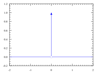
This seems like a good time to introduce the dirac delta function, which is a weird function that exemplifies the above consideration: it has zero variance, and is 0 everywhere apart from x=0, but it still integrates to 1:

It’s useful for denoting very short events in time – we can use it to denote a spike (action potential) in a neuron, for instance.

Covariance

An important concept: how much two variance in two variables relate to one another (correlation is the covariance corrected for the magnitude of each variable).

This is similar to calculating the variance (see above), but we sub in another variable instead of squaring everything:

$Cov(f(x),g(y)) = \mathbb{E}[(f(x) - \mathbb{E}[f(x)])(g(y) - \mathbb{E}[g(y)])]$

Covariance will be positive if two things tend to vary in the same direction (e.g. height and weight) and negative if two variables tend to vary oppositely (e.g. height and number of books you have to stand on to reach the top shelf). Note that covariance is a linear construct: two variables can be related in a funky non-linear way, and still have zero covariance.

A bunch of distributions

Bernoulli

A discrete probability distribution for describing the probability over a single binary variable, the most classic example of which would be heads or tails on a coin. It has a single parameter, $\phi$ ,which says how likely the binary variable is to attain state 1 (for an unbiased coin, $\phi$ is 0.5).

The multinoulli distribution does the same thing over k states.

Gaussian (=normal)

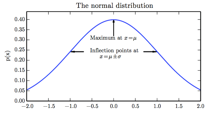
The old favourite. Random variables tend to the Gaussian distribution due to the central limit theorem . Despite being exceedingly common, you may never have actually seen the formula written down:

$N(x;\mu,\sigma^2)=\sqrt{\frac {1}{2\pi\sigma^2}}exp(-\frac{1}{2\sigma^2}(x-\mu)^2)$

Phew, what a mouthful. $\mu$ is the mean, $\sigma$ is the standard deviation ( $\sigma^2$ =variance).

They have a nice figure in the book (3.1):

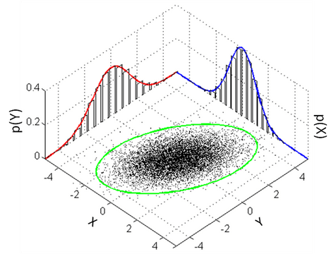
We can bang in lots more variables to the Gaussian distribution to produce a multivariate normal distribution. This involves replacing our scalar mean with a vector of means (μ –> μ) and our variance with a covariance matrix, Σ.

An example plotted for 2 dimensions;

(from Wikipedia)

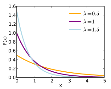
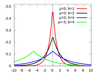
Exponential & laplace

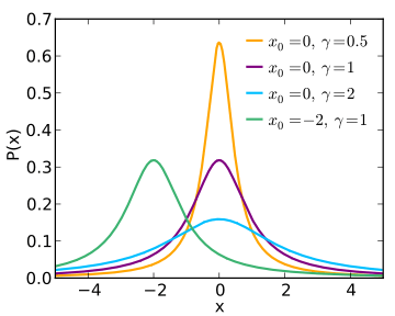
Used to give us nice and spiky distributions. For (negative) exponential, this spike is at 0, whereas the laplace distribution gives us the ability to shift it around based upon the point μ. Both are characterised by a steepness parameter γ (b in the laplacian graph):

Exponential:

NB Exponential is a special subset of gamma distributions (which look a bit like a mixture between an exponential and a normal distribution- they have a peak, and a long tail).

Laplace:

(from Wikipedia)

A mixture of distributions

We can combine a multinoulli distribution with some set of the above to generate a distribution mixture. The multinoulli specifies which distribution we are likely to be in on each trial.

$P(x) = \Sigma P(c=i)P(x|c=i)$

Where P(c) is the probability distribution over component distributions. This tells us that the probability of obtaining a certain value (x) is a product of the probability that we are in a certain state, and the probability of x given that state.

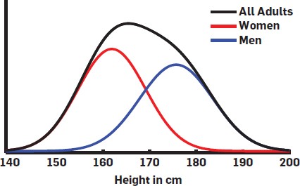
A common use of this is in Gaussian mixture models. We use these in neuroscience when we think that a population might be composed of multiple groups. For instance, the distribution of heights across the population is best described by two Gaussians, one for men, one for women. In this case gender is a latent, or hidden variable – an extra piece of information not inherent in the data, but which allows us to understand our data better.

(from Disentangling Gaussians)

Useful functions

When working with neural networks, we use functions which curtail the firing rates of our neurons to positive values (because neurons can’t fire at a negative rate).

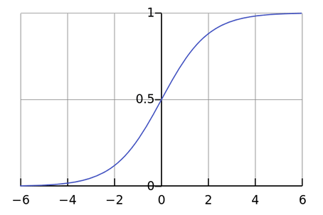
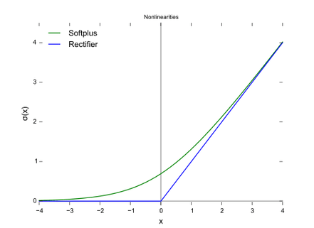
Two useful ones: the sigmoid (this is what everybody used to use) and the rectifier & soft plus (I believe these is more in fashion now).

Sigmoid

Rectifier & softplus

(from Wikipedia)

Transforming distributions

Sometimes we want to project one distribution through another. One common example from model-fitting: we want to fit a parameter in an unbounded space (-infinity to +infinity), but then when we use this parameter, we need to constrain to, for instance between 0 and 1 (if, for instance, we are fitting a learning rate). In this case, we’d fit the parameter then pass it through a sigmoid.

We can derive the new distribution by multiplying the original distribution by the derivative of the transformation:

q(x) = p(x) * g'(x)

Bayes rule

A favourite of ours, it’s:

$p(a|b) = \frac{p(b|a)p(a)}{p(b)}$

A derivation:

p(x,y) = p(x|y)p(y)

2. p(x|y) = p(x,y)/p(y)

Doing the same in reverse:

3. p(y,x) = p(y|x)p(x)

The substitute in p(y|x)p(x) for p(y,x) in eq. 2, and we get:

p(x|y)=p(y|x)p(x) / p(y)

Woohoo!

A little bit of information theory

Information is defined as the amount of uncertainty we reduce when we learn something. If you know something already, being told it again has an information content of zero. If something is very unlikely and you find out it has occurred, you gain a lot of information. If something was very likely and you find out it has occurred, you gain a little information.

Formally:

$I(x) = -logP(x)$

So information is negatively related to probability: the more probable something is, the less we learn when we find out the outcome. Depending upon the type of logarithm you use here, information comes in different units: nets (for the natural log), or bits or shannons (log2).

We quantify the amount of uncertainty in a whole probability distribution (rather than merely associated with a single event, x) using the Shannon entropy:

$H(x) = \mathbb E {}}_{x\sim P}[I(x)]$

Which is basically the expectation (i.e. the average) of the information.

Kullback-Leiber (KL) divergence

A phrase which many have heard and, I suspect, few have understood. The KL-divergence quantifies the difference between two distributions. More precisely, it quantifies how much information we use if we try and approximate one distribution with another distribution. Interestingly, it’s not symmetric – the amount of info we lose when we use A to approximate B ≠ the amount of info lost when we use B to approximate A.

It has quite a simple formula:

$D_{KL}(P\parallel Q) = \mathbb{E} _{x \sim P}[logP(x)-logQ(x)])}}$

Basically the average difference in probabilities of observing each sample based upon the two distributions!

Note that this means that the KL captures both differences in means and variances of distributions.

A related concept is the cross-entropy:

$Cross Entropy (x,y) = p(x,y)log\frac{p(x,y)}{p(x)p(y)}$

If the two variables are completely independent, p(x,y) = p(x)p(y) [that’s the product rule], and we end up with log(1), which is 0. If p(x,y) > p(x)p(y). then the joint probability is higher than the product of the independent probabilities, implying that the variables are related- and yielding a positive cross entropy.

Graphical models

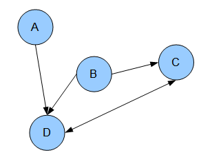
Basically a way of drawing out probabilistic relationships. They consist of nodes (distributions, or functions), and edges (links between them).

They can be directed, in which case we are visualising conditional relationships, or they can be undirected, which allows us to mix in non-probabilistic functions.

In undirected models, nodes which are linked together by edges are referred to as cliques.

A directed graph:

(Wikipedia)

One common usage is to describe transitions in a Markov model:

(Wikipedia)

The advantage of having a graphical model is that it allows us to depict dependencies. If we learn these dependencies, then we save ourselves the effort of learning the whole covariance matrix across all of the variables. This is probably the kind of trick the brain uses to make things easier…