Deep Learning Book Chapter 3: Numerical Computation

June 20, 2016

This chapter was a bit of pot-pourri of things the authors wanted to tell us before we got on to machine learning proper. Much of it was straightforward, and then there were a few stingers, such as the bits about directional gradients.

Typical problems we need to be aware of in using a digital computer to do analogue stuff

Underflow & overflow

Underflow: where very small numbers –> zero, and overflow: big ones –> zero.

For instance, for a softmax:

$softmax(x_i)= \frac{exp(x_i)}{\sum_{j=1}^{n} exp(x_j) }$

We have an issue if our x’s are very negative, because by exponentiating them we push them very close to zero, possibly resulting in underflow. Similarly, with huge x, we might get overflow. We can do a bit of normalization to overcome this: by subtracting max(x), we don’t change the computation, but we ensure that in the numerator everything is <0, and in the denominator, at least one of the entries is exp(0)=1, which means we’re not going to get underflow!

Poor conditioning

This is where we have a matrix -remember, we can usefully think of matrices as transformations– which responds very drastically to small changes in input – precisely the kind of small changes we might induce by digitizing an analogue variable.

Conditioning is defined by a condition number, which are calculated from the ratio of the maximum to the minimum eigenvalue. High condition numbers are problematic.

Gradient descent (vanilla)

Gradient descent is the most obvious weapon in our arsenal for minimising some function, which we want to do a lot. Typically this function is a cost function of some kind – and by minimizing it, we maximise some measure of ‘goodness’ of our model.

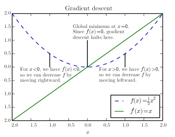
In gradient descent, we work out the derivative of our function to be minimized, then take small steps in the direction opposite to the gradient.

$Cost= y(x)$

$Gradient = \frac{d(y)}{d(x)}$

Why do this? Well, if we’re in a region where the gradient is positive, this means that increasing X with increase Y. So we don’t want to do this (we’re minimising Y, remember). So we should decrease X.

Conversely, if dy/dx is negative, then if we increase X, we’ll decrease Y. So that’s exactly what we should do: increase X.

Nicely illustrated by Figure 4.1 from the book: $[\frac{\delta(y)}{\delta(x)} \\ \frac{\delta(y)}{\delta(x)} \\ \frac{\delta(y)}{\delta(x)} ]$

Gradient descent (partial derivatives)

What if we have multiple independent variables, and our cost is a function of lots of them:

$Cost= y(x_1,x_2,x_3)$

Well, we can basically do the same trick, but use partial derivatives. What results is a gradient vector:

$[\frac{\delta(y)}{\delta(x_1)} \\ \\ \frac{\delta(y)}{\delta(x_2)} \\ \\ \frac{\delta(y)}{\delta(x_3)} ]$

The gradient vector is denoted as : $\bigtriangledown_xf(x)$

In both the single and multiple gradient case, how much we move in the direction of the gradient is a matter of choice: we define a learning rate or step size which describes how much to jump at each step. Too small and everything will be super slow, and too large, and you risk missing the minimum.

Stationary points

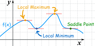
Stationary points are where the gradient = 0. They can be maxima, minima, or saddle points, best illustrated graphically:

Credit here

We can discriminate between these with the second derivative; positive second derivatives imply a minimum, negative second derivatives a maximum, and zeros a saddle point. This is straightforward in two dimensions, but for higher dimensional problems, we need to turn to the Jacobian.

Jacobians and Hessians

Confusing terms, these. A Jacobian is a matrix filled with differentials. The gradient is itself the Jacobian of the original function.

A Hessian is a certain kind of a Jacobian: it’s the Jacobian of the gradient, when we have multiple variables and the gradient is a vector of partial derivatives.

So:

$y=f(x_1,x_2,x_3) <-- original function \\ [\frac{\delta(y)}{\delta(x)} \\ \frac{\delta(y)}{\delta(x)} \\ \frac{\delta(y)}{\delta(x)} ] <-- Jacobian(y) = gradient \\$

$[\frac{\delta^2(y)}{\delta(x_1)^2} \ \ \ \ \frac{\delta^2(y)}{\delta(x_1) \delta(x_2)} \frac{\delta^2(y)}{\delta(x_1) \delta(x_3)\\ ...... ]$ <— Jacobian ( $\bigtriangledown_xf(x)$ ) = the Hessian (incomplete; my Latex editor started playing up when I went to multiple lines.).

Why do we care about the Hessian?

Two reasons, so far as I can make out:

We can use it to figure out the nature of a multidimensional stationary point, by referring to the eigenvectors:
- All positive = minima [Hessian = positive definite]
- All negative = maxima [Hessian = negative definite]
- Mix = saddle point
We can use Newton’s method to do second-order gradient descent

Newton’s Method

Traditional gradient descent allows us to chug down our gradient, but it can be very slow.

Newton, widely held to be a pretty clever chap, described a neat method for doing zero-finding for a function – that is, finding the value of x where f(x) = 0. This means that if we use f’ instead of f, and find the value of x where f'(x) =0, we’ve done minimisation. To do this, we need the Hessian, because this provides us with the ‘gradient of the gradient’, so to speak.

Using Newton’s method for zero-finding

Newton’s method gives us an iterative way of finding better and better approximations to the roots of y(x).

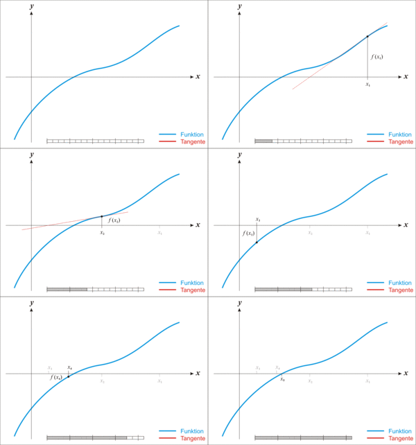
Graphically, here’s how it works:

take a value of x, let’s call it $x{_n}$
take the tangent to the line at this point
find the point where the tangent crosses the x-axis
this is your new x: $x_{n+1}$

And repeat. This is illustrated below (from Wikipedia):

Numerically, the update formula is:

$x_{n+1} = x_n - \frac{f(x_n)}{f'(x_n)}}$

How does this relate to the graphical intuition above? Well, the formula for a tangent is

$y= f'(x) (x-x_n)+f(x_n)$

And we’re going to find the point where y=0, and solve for x= $x_{n+1}$ :

$0 = f'(x_n)(x_{n+1}-x_n) + f(x_n)\\ \frac{-f(x_n)}{f'(x_n)} = x-x_n\\ x_{n+1} = x-\frac{f(x_n)}{f'(x_n)}$

Now clearly, if we want to do minimisation rather than zero-finding, all we have to do is substitute f for f’.

So we end up with

$x_{n+1} = x_n - \frac{f'(x_n)}{f''(x_n)}}$

And $f''(x_n)$ is the Hessian.

Cool properties of Newton’s method

Newton’s method allows us to jump down the gradient rather than rolling. In particular, if our function is second-order, that means the differential is first-order, and Newton’s method will find the local minima in a single jump!

Constrained optimisation

Disclaimer: I’m not sure I understand this very well and I don’t think it’s terribly important (right now), so apologies if it’s not very clear

The Krush-Kahn-Tucker (KKT) approach is useful for adding constraint to optimizations. It’s a development of the Lagrangian method, which allows you to specify some equality; KKT allows you to specify inequalities too.

We can use it when we want to minimise/maximise some function $f(x,y,...n)$ , with some constraints $g(x,y,...n) = c$ , where $c$ is some constant. Note that we can only use it when the constraining function is also a function of the same input variables i.e. $x,y,...n$ match for $f$ and $g$ .

Concrete example – from Khan Academy’s peerless summary:

Let’s say we have a simple function:

$f(x,y) = 2x + y.$

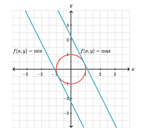
We want to maximise it, but we’re only interested in points on a circle, where:

$x^2 + y^2 = 1.$

To rephrase our question: we want to ask ‘where, on my circle, is the function f greatest’?

This is equivalent to projecting our circle onto a linear plane (defined by the function $f$ ):

Ok. now for the clever bit.

Solving our constrained optimisation involves finding the maximum of function $f$ whilst still meeting our constraining criterion, $g$ . It turns out that the values of $f(x,y)$ that we’re looking on are contour lines of $f$ which are tangential to the function $g$ .

Credit: Khan Academy.

Now: if two contour lines are tangent, this means that their gradients are parallel i.e. they share a direction (the vector might have different lengths or directions, but that doesn’t matter).

Let $x_0$ $y_0$ be a point where the two are tangent. In that case:

$\bigtriangledown f(x_0,y_0) = \lambda\bigtriangledown g(x_0,y_0)$

I.e. the gradient of $f$ can be obtained from that of $g$ by multiplication by some constant $\lambda$ . This is the Lagrange multiplier.

Lagrange’s formulation thus provides a helper function which helps us crack open our constrained optimisation.

$L(x,y,\lambda) = f(x,y) + \lambda (g(x,y)-c)$

Where $L$ is a Lagrangian, $\lambda$ is our Lagrange multiplier, and $c$ is the constraint upon $g$ (i.e. $g(x,y) = c$ ).

I think that by bringing $\lambda$ inside our optimisation, we elevate it from being a ‘soft constraint’, for which we have to describe some penalty function, to a ‘hard constraint’ – we directly optimise for lambda.